Part 2: Working with a single scan

Russell Rogers

Geological Survey Ireland

In CoreSpecViewer: Start with a single scan

Open a hyperspectral core scan

Launch CoreSpecViewer using the installation guide on the repository page.

  • Note that you are on the Raw page, one of four pages
  • Open the load dialogue, by clicking the open button at the top left of the interface.
  • Examine the different data formats it can open.
  • Open the Raw Lumo output directory from the downloaded data.

The following slides all assume that you are working with hole 100131808811W500 box 103. The output descriptions will not make any sense if you are using a different scan.

Data Correction

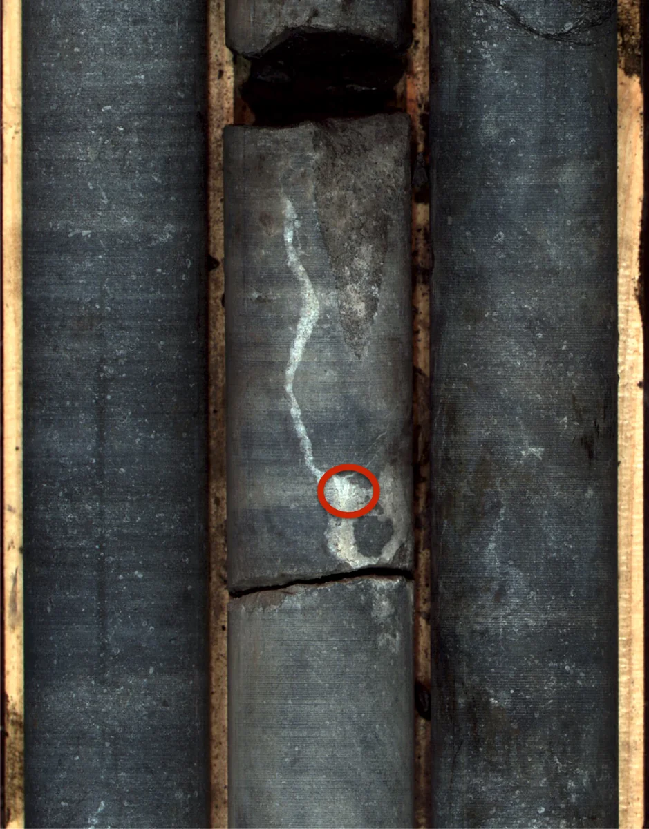
The area circled in red is part of a calcite vein.

A pixel from this vein will be used in the following examples.

Data Correction
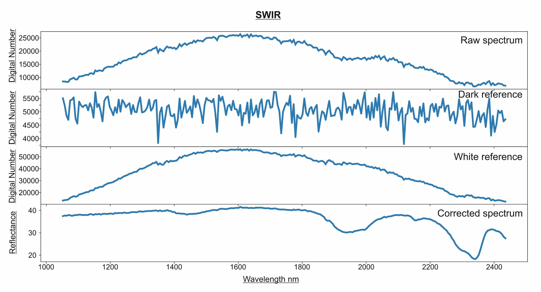
\[ \text{Reflectance (%)} = \frac{\text{Sample} - \text{Dark}}{\text{White} - \text{Dark}}\times 100 \]

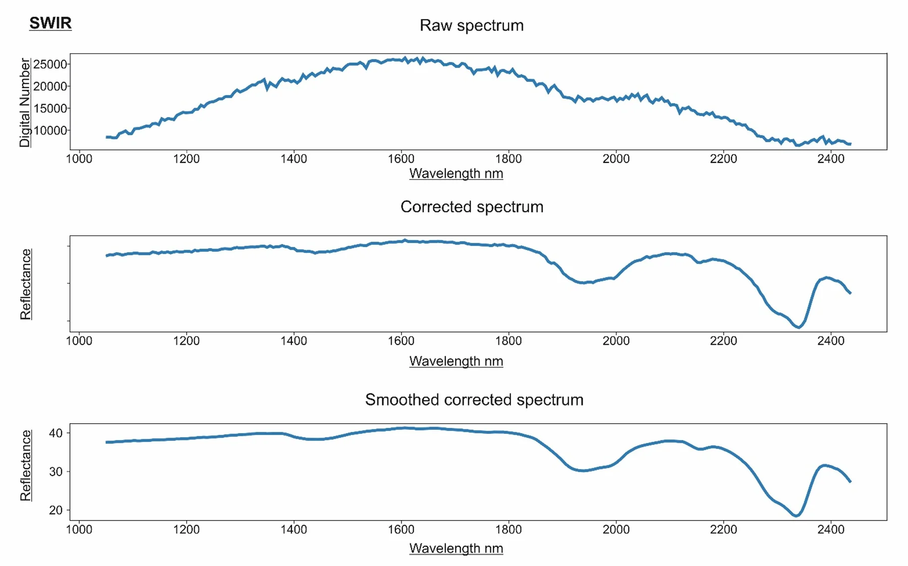
The image shows the data from a pixel of the calcite vein in the raw data, a spectrum of the dark reference and a spectrum of the white reference. The image is corrected to reflectance using the formula by CoreSpecViewer on load.

In CoreSpecViewer: Open and Process

Raw page:

  • Double-click a few pixels to see how directly you can interrogate the image.
  • Click Auto-crop.
  • Click Undo
  • Manually crop the image.
  • Click Process.

Data Correction

Our calcite pixel

By clicking Process CoreSpecviewer takes the cropped extent of the reflectance corrected scan and performs smoothing using the supplied parameters (default is Savitzky-Golay, window=11, polynomial-order=2)

Convex Hull Quotient
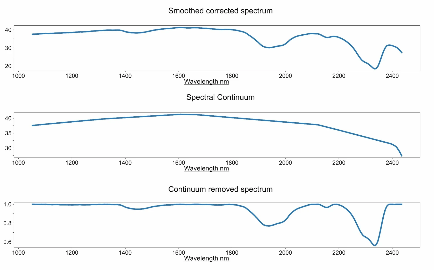
As further part of the Process operation:

  • Continuum, or convex hull, is calculated.
  • Spectrum is divided by the convex hull.
  • All values are now 0–1.
  • Features are more identifiable and spectra more comparable.

In CoreSpecViewer: Processed Data

Visualise page:

  • Look at the cached products table.
    • These are the pre-calculated derived products from Process
  • Double-click some pixels.
    • This is the smoothed reflectance spectrum of the clicked pixel
  • Right-click some pixels.
    • This is the continuum removed reflectance spectrum of the clicked pixel
  • Examine the metadata available through the Info button.
  • Click the Settings button.
    • These are the preset parameters that were used during processing.

In CoreSpecViewer: Masking

Visualise page:

  • Click New Mask — select a pixel of the core box itself.
  • Enhance Mask — select a different pixel of the box.
  • Freehand Mask — draw a polygon.
  • Create a good core mask, marking non-core pixels.

In CoreSpecViewer: Segmentation

Visualise page:

  • Look at the box convention in Settings.
  • Click Calc Stats.
  • Open the Segments image.
  • Click Unwrap Preview.
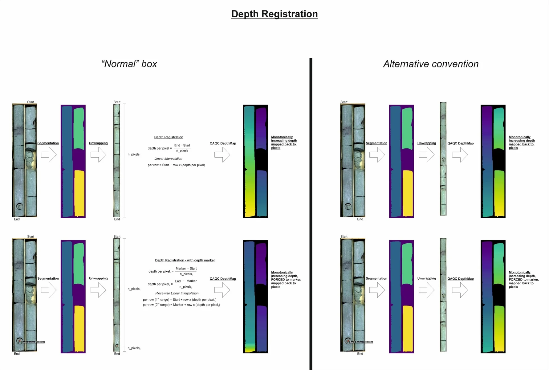
  • Open the DepthMap image from the products table

Unwrapping and Depth Registration

In CoreSpecViewer: Depth Registration

Visualise page

  • Check that your DepthMap is monotonically increasing in the correct convention.
  • Click the Info button and check that the correct convention is embedded.
  • Click Save.

We now have a pre-processed data cube ready for interpretation.

In CoreSpecViewer: Spectral Exploration

Visualise page

  • Click Quick-cluster.
  • Use the default 5 clusters and 50 iterations.
  • Examine the map.
  • Double-click Cluster Centres.
  • In the cluster centres window, double-click a class to view its centre.

In CoreSpecViewer: Spectral Exploration

Visualise page:

  • Click Band Maths.
  • Run some indices in the dialogue. Using the equation to name the product is recommended.

Examples:

R2320
R2350
R2250
R2250 / interp(R2150, R2350)

Absorption Features

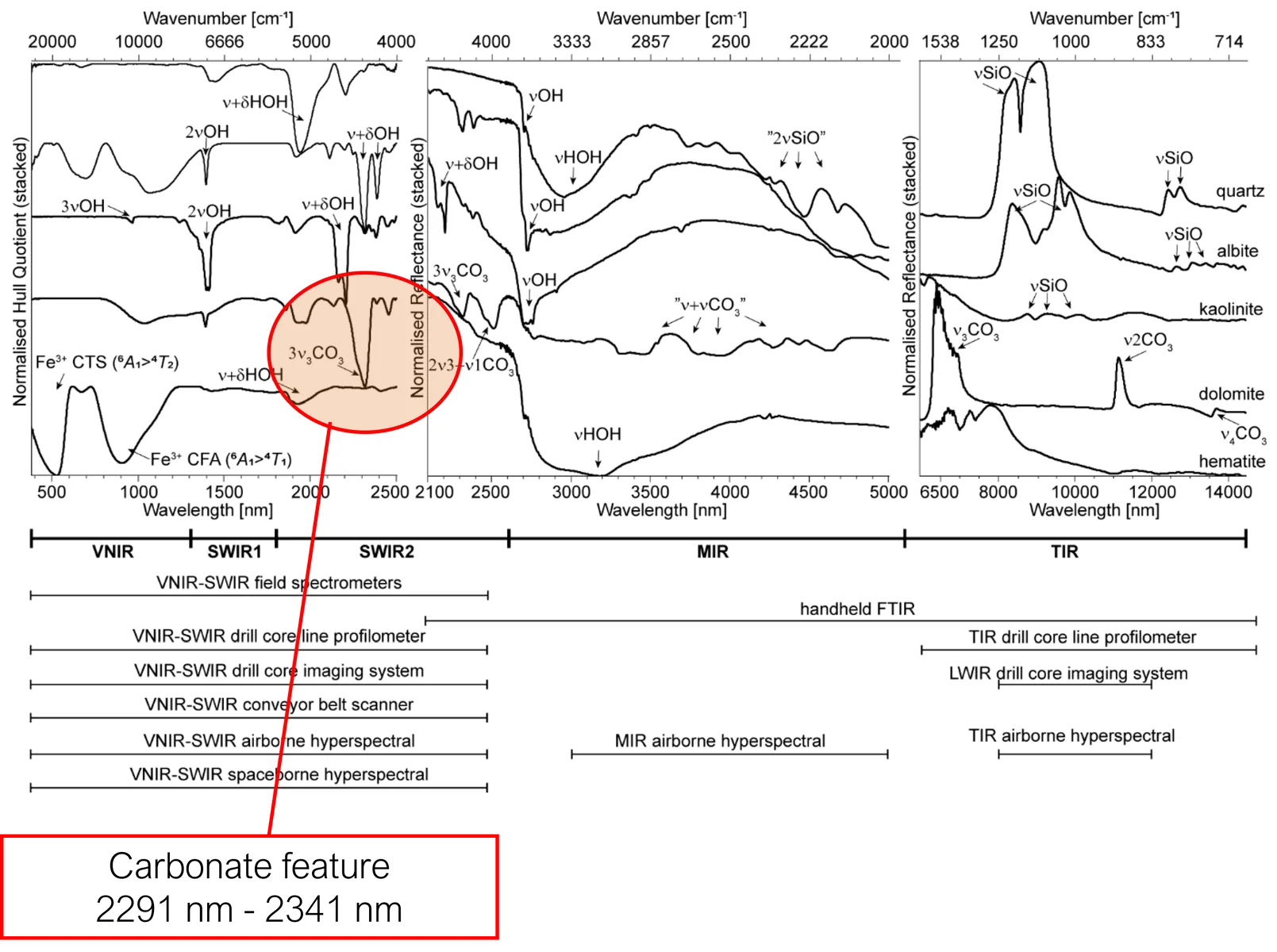
Reflectance spectra of major rock-forming minerals in the 500–14,000 nm wavelength region.

Figures taken from Laukamp et al. (2021): Mineral Physicochemistry Underlying Feature-Based Extraction of Mineral Abundance and Composition from Shortwave, Mid and Thermal Infrared Reflectance Spectra. Minerals, 11(4), 347.

Absorption Features
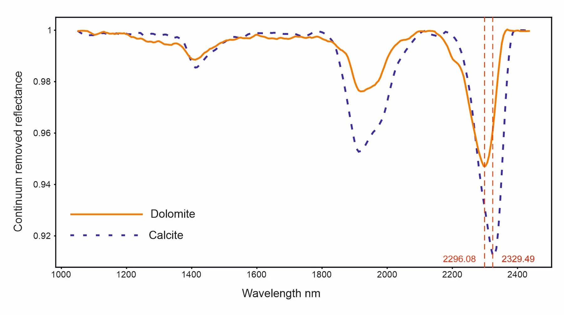
From library reference spectra and published research, the 2300 nm feature is known to vary with carbonate composition.

  • Longer wavelengths: more Ca-rich.
  • Shorter wavelengths: more Mg-rich.

Spectra taken from JPL spectral library. Meerdink, S. K., Hook, S. J., Roberts, D. A., & Abbott, E. A. (2019). The ECOSTRESS spectral library version 1.0. Remote Sensing of Environment, 230, 111196.

Feature Extractions
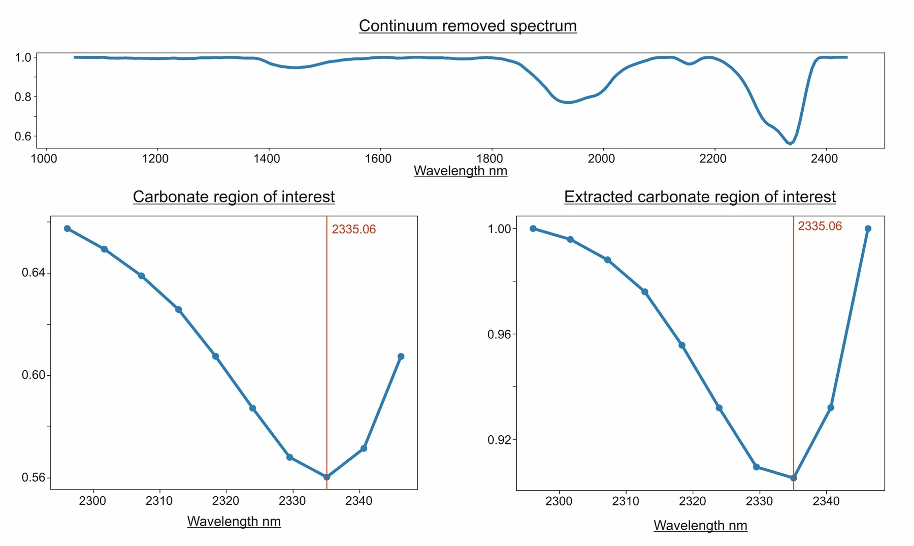
  • Top continuum removed full spectral range
  • Left: carbonate feature region plotted from the continuum-removed curve.
  • Right: continuum removed from the feature region of interest only.

NB: different curve shape, but same minumum on measured band centre.

Feature Extractions: Inter-band Fitting Minimum
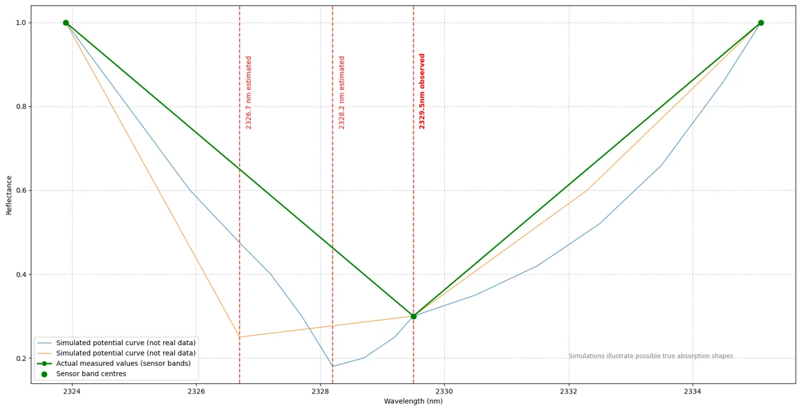
Many curves, with very different minima, can fit the measured data.

Feature Extractions: Inter-band Fitting Minimum
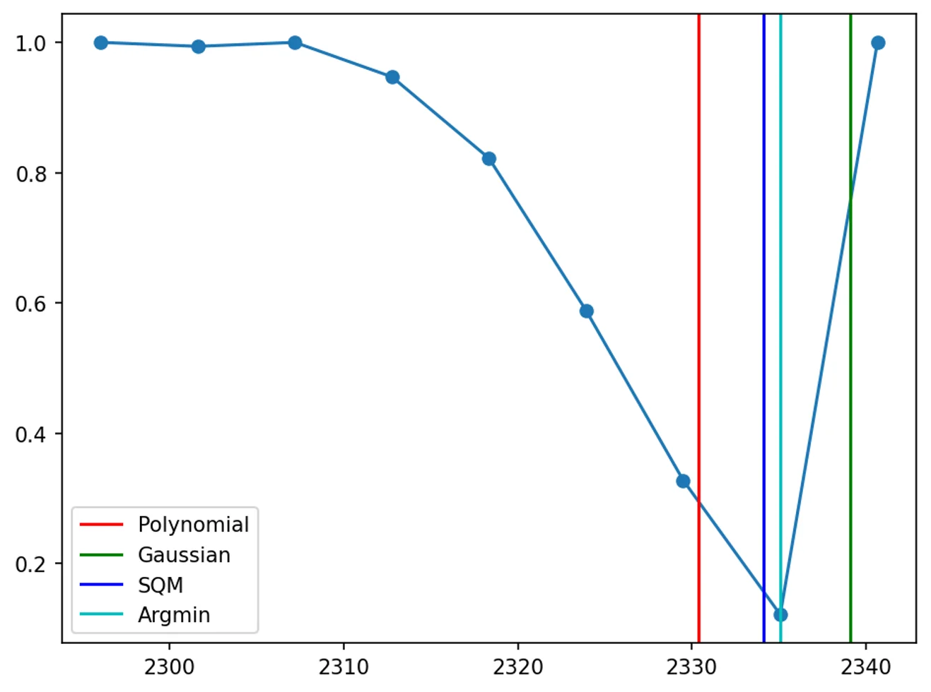
  • Argmin — simple band-centre minima.
  • SQM — quadratic polynomial fitting¹.
  • Polynomial — higher-order polynomial fitting².
  • Gaussian — multiple Gaussian curve fitting².

CoreSpecViewer defaults to Polynomial fitting, which can be changed in the source.

¹ Rodger, A., Laukamp, C., Haest, M. & Cudahy, T. (2012). A Simple Quadratic Method of Absorption Feature Wavelength Estimation in Continuum Removed Spectra. Remote Sensing of Environment, 118, 273–283.

² Thiele, S. T. et al. (2021). Multi-scale, multi-sensor data integration for automated 3-D geological mapping. Ore Geology Reviews, 136, 104252.

Feature Extractions: Defined Ranges
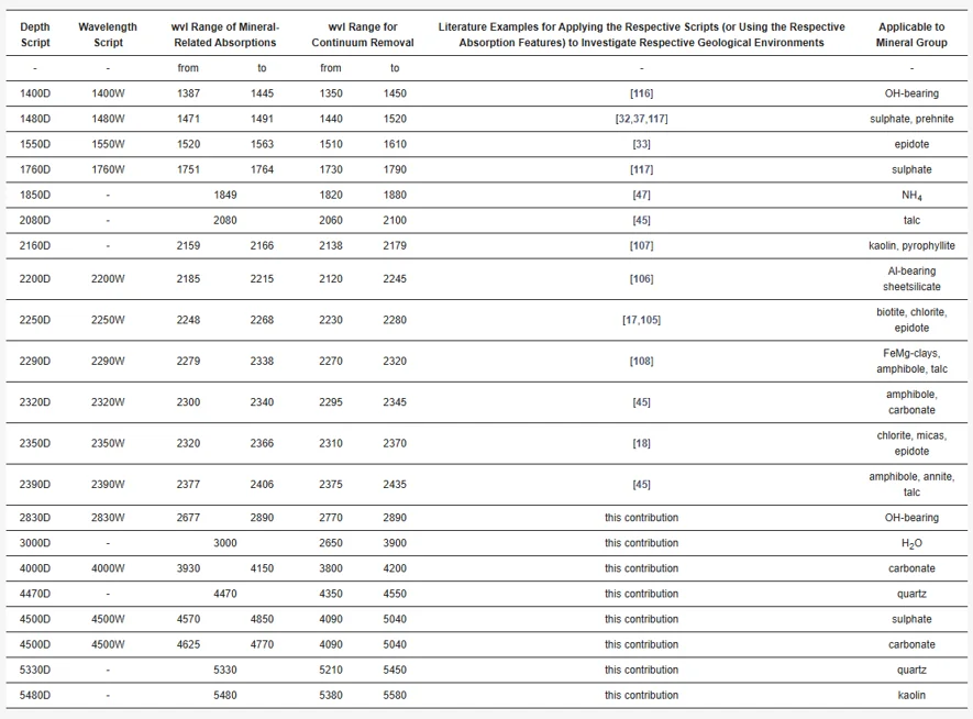
Table 5 from Laukamp et al. (2021). Values for these features are hard-coded into CoreSpecViewer.

Laukamp, C. et al. (2021). Mineral Physicochemistry Underlying Feature-Based Extraction of Mineral Abundance and Composition from Shortwave, Mid and Thermal Infrared Reflectance Spectra. Minerals, 11(4), 347.

In CoreSpecViewer: Feature Extractions

Visualise page

  • Click Features and in the dropdown select:
    • 2250W
    • 2350W
    • 2320W
  • Examine the feature maps.
  • Right-click different feature-map regions to examine spectra.

In CoreSpecViewer: Library and Spectral Correlation

The following instructions assume that you are using the Ecostress library version distributed with CoreSpecViewer.

Library page:

  • Sort the library by mineral name.
  • Scroll to the bottom to load every mineral.
  • Type C, a to jump to calcite.
  • Double-click and right-click a few calcite exemplars.
  • Click Filter to Current Band Range.
  • Examine Calcite [116]; click Correlate on the Library page and look at the coefficient values in the image.
  • Examine Dolomite [124]; click Correlate on the Library page and look at the coefficient values in the image.

In CoreSpecViewer: Library and Collections

Library page:

  • Select Calcite [116], click Add to Collection, name it Demo1.
  • Select Dolomite [124], add to collection Demo1.
  • In the dropdown, select Demo1.

In CoreSpecViewer: Mineral Mapping

Visualise page:

  • Click Correlations.
  • Select MineralMap Pearson (Winner-takes-all).
  • Choose the in-range collection.
  • Examine the mineral map.
  • Click Correlations again.
  • Select MineralMap Pearson (Winner-takes-all).
  • Choose the Demo1 collection.
  • Examine the mineral map.

In CoreSpecViewer: Mineral Mapping

Library page:

  • Examine Chlorite [1055]; click Correlate and inspect coefficient values.
  • Add Chlorite [1055] and the contents of Demo1 to Demo2.

Visualise page:

  • Run Pearson correlation on Demo2 and examine the mineral map.
  • Right-click gaps to inspect their spectra.

Library page:

  • Add Illite [969] and the contents of Demo2 to Demo3.
  • Run Pearson correlation on Demo3 and examine the mineral map.

In CoreSpecViewer: Mineral Mapping

Library page:

  • Add Montmorillonite [1007] and the contents of Demo3 to Demo4.
  • Click into montmorillonite-coloured spectra.
  • Click Correlations → Select Range → Pearson → 2000 to 2600.
  • Examine the mineral map.
  • Run Features extraction on 1900W.
  • Examine the map.

In CoreSpecViewer: Mineral Mapping

Visualise page:

  • Click Correlation → MineralMap SAM (winner-takes-all) → Demo4.
  • Examine the mineral map.
  • Click Correlations → Select Range → SAM → 2000 to 2600.
  • Examine the mineral map.

In CoreSpecViewer: Saving and Exporting

Visualise page:

  • Click Save.
  • Click Generate Images.
  • Click Generate Box Report.

Single Scan Interpretation: Take-aways

  • Information-dense datasets.
  • Many tools to interpret the data.
  • A combination of many approaches and geological knowledge of the core is the best way to extract the most understanding from the data.
  • ML models, while not covered here, lack many of the weaknesses of this holistic approach, but introduce new weaknesses of their own.
  • Be wary of hyperspectral mineral maps, even if you know the exact methods used to produce them.